Round to Odd

Added: November 19, 2025
Last updated: November 26, 2025

When writing numerical programs, rounding is a subtle but important aspect that can significantly affect the accuracy and stability of computations. In particular, rounding twice at different precisions might introduce unexpected errors. For example, under the nearly universal round to nearest, ties to even (RNE) rounding mode, adding 1.00000011 and 5.96046447e-8, and rounding directly to a single-precision floating-point value yields 1.00000012; but first rounding to a double-precision floating-point value then to a single-precision floating-point value yields 1.00000024. This phenomenon is known as double rounding.

The double rounding problem means that a high-precision reference cannot be used to verify the correctness of lower-precision implementations, even for a single operation. For example, naively using double-precision arithmetic to verify single-precision results is not enough to ensure correctness: double rounding may cause the reference result, rounded to single-precision, to disagree with the correctly-rounded single-precision result. When developing correctly-rounded implementations of floating-point functions, double rounding implies that we cannot simply compute the result at higher precision and then round it to the target precision. In the worst case, a correctly-rounded implementation must be specifically designed for each target precision, adding significant time and complexity to the implementation and verification effort.

Across the literature on floating-point arithmetic, one rounding mode offers a solution to double rounding: round to odd (RTO). This blog post covers the common rounding modes, and the definition and properties of round to odd. Finally, it concludes with the essential property of round to odd: safe re-rounding.

Floating-Point Numbers

To begin, I’ll briefly review floating-point numbers. Floating-point numbers are numbers represented in the form:

\[(-1)^s \cdot c \cdot 2^{exp}\]

where $s \in \{0, 1\}$ is the sign, $c \in \mathbb{Z}_{\geq 0}$ is the significand, and $exp \in \mathbb{Z}$ is the (unnormalized) exponent. The fewest number of digits that can represent $c$ is called the precision, $p$, of the number: if $c > 0$, then $2^{p - 1} \leq c < 2^p$. Alternatively, we can represent floating-point numbers in normalized form:

\[(-1)^s \cdot m \cdot 2^e\]

where $1 \leq m < 2$ is the mantissa and $e \in \mathbb{Z}$ is the (normalized) exponent. The relationship between the two forms is given by the equations:

\[c = m \cdot 2^{p - 1}\]

and

\[exp = e - (p - 1).\]

For example, we can represent $1.25$ using 3 bits of precision by $101 \cdot 2^{-2}$ and $1.01 \cdot 2^{0}$ in unnormalized and normalized forms, respectively.

The IEEE 754 standard extends floating-point numbers to include special values: including negative zero, $-0$; positive infinity, $+ \infty$; negative infinity, $- \infty$; and Not a Number, $\mathrm{NaN}$. Number formats define discrete sets of floating-point numbers that approximate real numbers.

A rounding operation maps real numbers to representable values of a number format according to rounding modes. Rounding modes determine which floating-point value to choose in cases where the real number cannot be represented exactly. There are several rounding modes in use today. For example, the IEEE 754 standard [1] defines five rounding modes: round to nearest, ties to even (RNE); round to nearest, ties away from zero (RNA); round to positive infinity (RTP); round to negative infinity (RTN); and round toward zero (RTZ).

Correctly-Rounded Functions

Rounding extends naturally to real-valued functions through correctly-rounded functions. We say that an implementation $f^{*}$ of a real-valued function $f$, is correctly-rounded if its result is the infinitely precise result of $f$, rounded to the target number format according to a specified rounding mode. We’ll only consider floating-point numbers with a fixed precision of $p$ digits, so I’ll denote the rounding operation in the style of Boldo and Melquiond [2] as $\mathrm{rnd}^{p}_{rm}$. Using this notation, the correctly-rounded implementation of $f$ in precision $p$ under rounding mode $rm$ can be expressed as:

\[f^{*} = \mathrm{rnd}^{p}_{rm} \circ f.\]

Requiring correct rounding has strong arguments [3]: it provides a clear specification for the behavior of $f^{*}$; it ensures reproducibility of results across different implementations of $f^{*}$; and it bounds the numerical error introduced by rounding.

We can now formalize the double rounding problem. In general, for precisions $p_2 < p_1$ and rounding modes $rm_1, rm_2$:

\[\mathrm{rnd}^{p_2}_{rm_2} \circ f \neq \mathrm{rnd}^{p_2}_{rm_2} \circ (\mathrm{rnd}^{p_1}_{rm_1} \circ f).\]

More succinctly, rounding operations do not compose:

\[\mathrm{rnd}^{p_2}_{rm_2} \neq \mathrm{rnd}^{p_2}_{rm_2} \circ \mathrm{rnd}^{p_1}_{rm_1}.\]

We will see that round to odd provides a solution to this problem.

Rounding Modes

Once we compute the infinitely precise result of $f(x)$ for a real number $x$, we need to round the result to get $f^{*}(x) = \mathrm{rnd}^{p}_{rm}(f(x))$. To illustrate the different rounding modes, we’ll consider three rounding modes: round to nearest, ties to even (RNE); round toward zero (RTZ); and round away from zero (RAZ).

If $f(x)$ is representable in the target number format, then no more work is needed: $f^{*}(x) = f(x)$. Otherwise, $f(x)$ lies between two representable floating-point numbers, which we’ll denote as $y_1 < f(x) < y_2$. To simplify the discussion, let’s assume that $y_1$ and $y_2$ are both positive, and that $y_1$ has an even significand $1XXX\ldots0$ and $y_2$ has an odd significand $1XXX\ldots1$.

The rules for each rounding mode are as follows:

RNE: round to the nearest representable number; if $f(x)$ is exactly halfway between $y_1$ and $y_2$, round to the one with an even significand $c$;
RTZ: round to the number in the direction of zero;
RAZ: round to the number in the opposite direction of zero.

Let’s first assume that $f(x)$ is closer to $y_1$ than to $y_2$.

rounding when $$f(x)$$ is closer to $$y_1$$

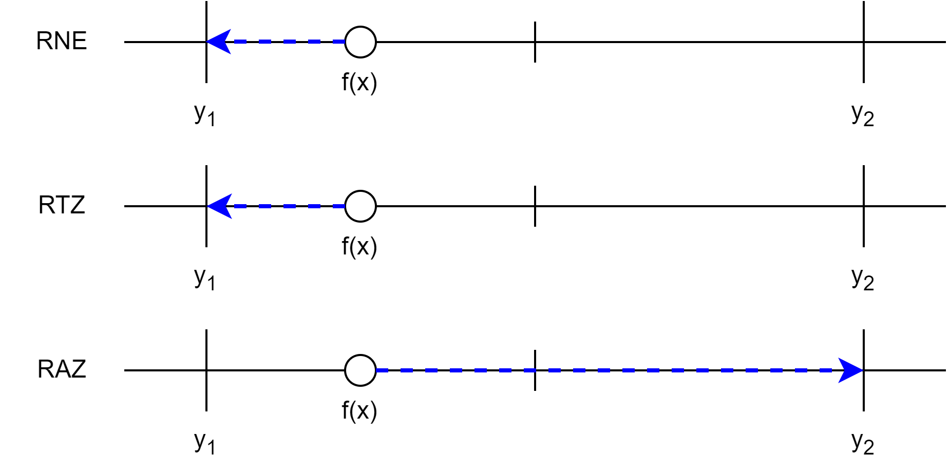
In this case, $f(x)$ rounds to

RNE: $y_1$ since it is the nearest representable number,
RTZ: $y_1$ since it is in the direction of zero,
RAZ: $y_2$ since it is in the opposite direction.

Now, let’s assume that $f(x)$ is closer to $y_2$ than to $y_1$.

rounding when $$f(x)$$ is closer to $$y_2$$

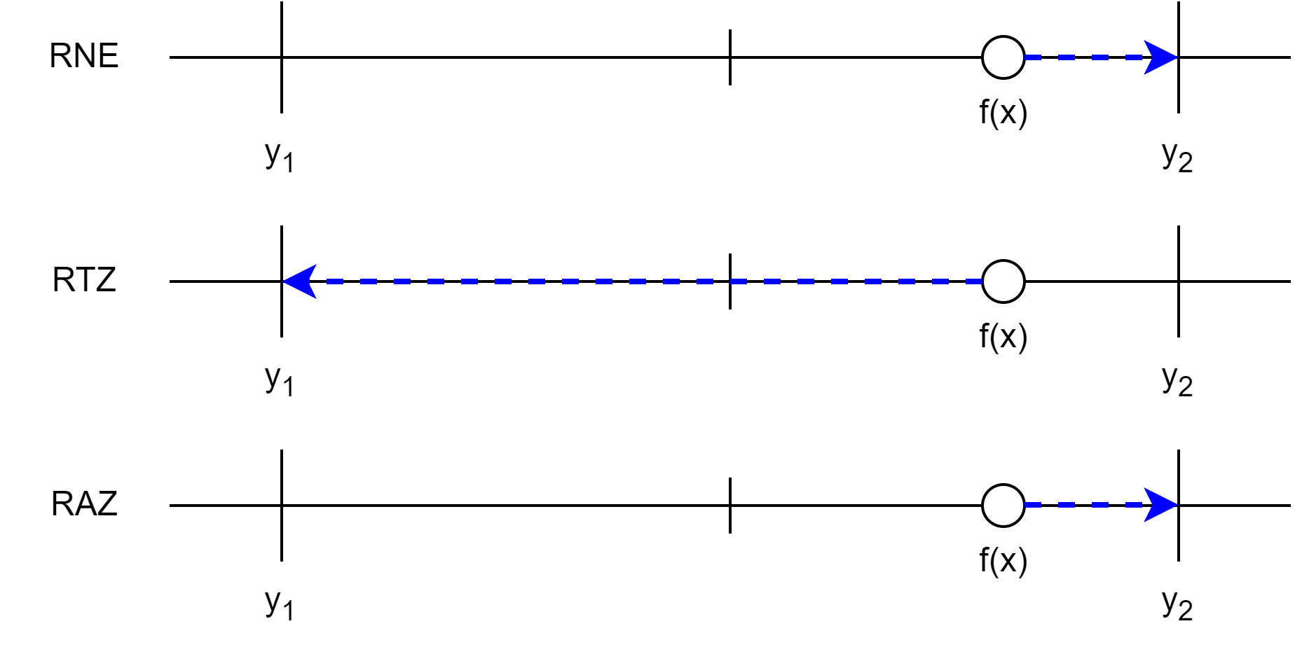
The only difference is that $f(x)$ rounds to $y_2$ under RNE, since $y_2$ is now the nearest representable number.

Finally, let’s consider the case where $f(x)$ is exactly halfway between $y_1$ and $y_2$.

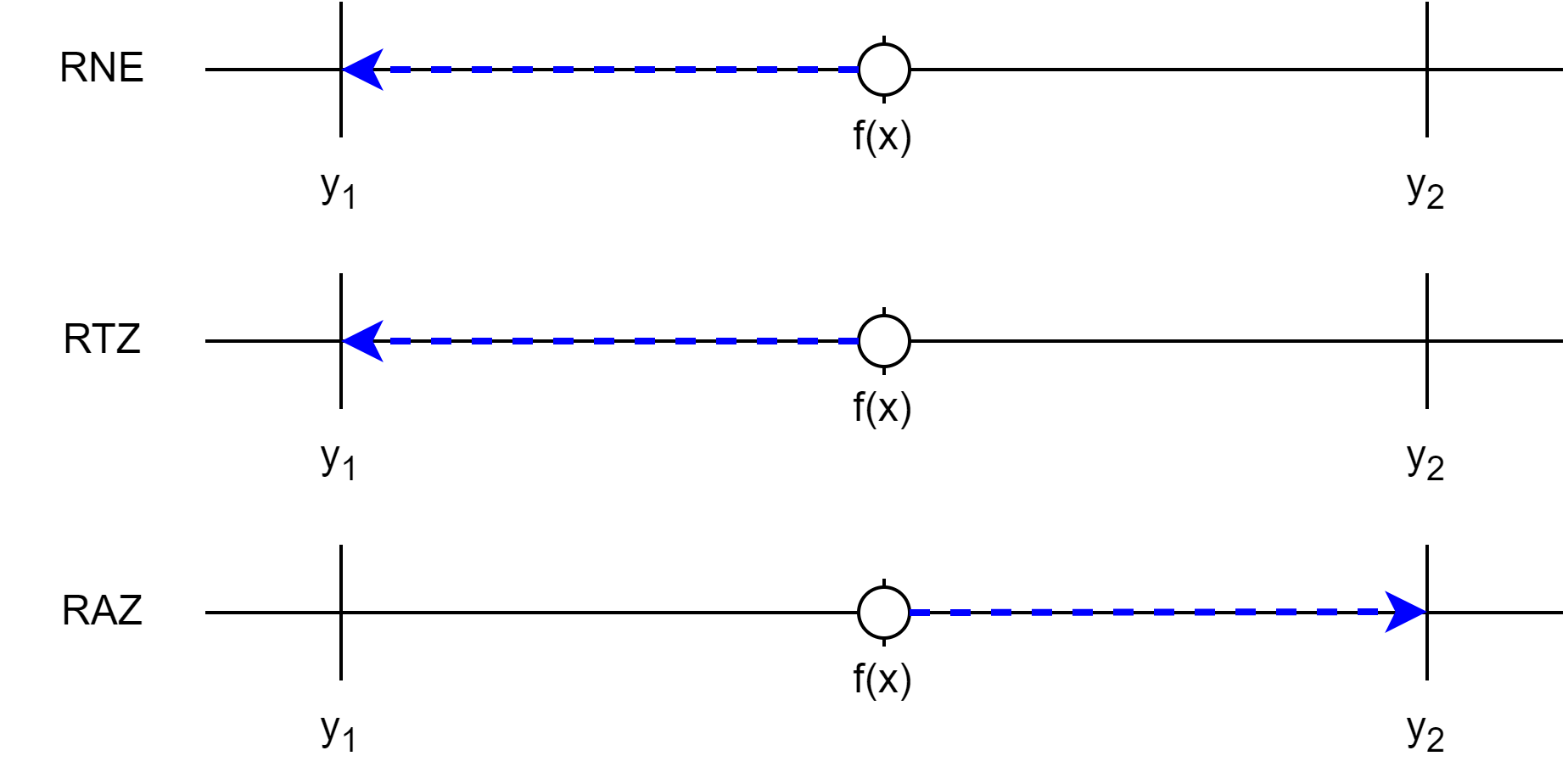
rounding when $$f(x)$$ is equidistant to $$y_1$$ and $$y_2$$

Rounding under RNE will tie-break to the even significand, in this case, $y_1$. Under RTZ and RAZ, the result is the same as before: RTZ rounds to $y_1$ and RAZ rounds to $y_2$.

Other rounding modes like round to nearest, ties away from zero (RNA); round to positive infinity (RTP); and round to negative infinity (RTN) can be analyzed similarly. RNA is similar to RNE, except that it tie-breaks to the representable value away from zero. RTP rounds towards positive infinity: it is the same as RAZ for positive numbers, and RTN is the same as RTZ for positive numbers. RTN is the opposite of RTP.

Round-to-Odd

Round to odd is only a slight adaptation of the rounding modes we’ve seen so far. Like before, if $f(x)$ is representable in the target number format, then no rounding is required: $f^{*}(x) = f(x)$. Otherwise, $f(x)$ lies between two representable floating-point numbers, which we’ll again denote as $y_1 < f(x) < y_2$. Under RTO, we round to the representable number with an odd significand $c$. In our example, this means that we always round to $y_2$.

Round to odd should not be confused with round to nearest, ties to odd (RNO); the rounding mode that uses the opposite tie-breaking rule of round to nearest, ties to even (RNE). RTO is not a nearest rounding mode. For RNE and RNO, the “even” (and “odd”) refers to the tie-breaking rule when $f(x)$ is exactly halfway between $y_1$ and $y_2$. For RTO, the “odd” refers to the rule whenever $f(x)$ is not representable.

rounding $$f(x)$$ under RTO

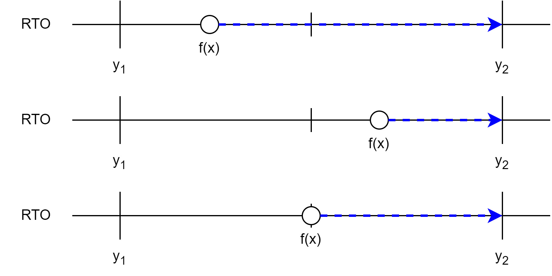
Like RTZ and RAZ, any value between $y_1$ and $y_2$ rounds to the same result, in this case, $y_2$. On this example, round to odd doesn’t seem too interesting.

However, examining its behavior on a different example reveals a key property of RTO. Let’s zoom out and consider the next representable floating-point number after $y_2$, which we’ll denote as $y_3$. In a floating-point number format with one fewer bit of precision $p - 1$, $y_1$ and $y_3$ would be adjacent representable numbers, and $y_2$ would be the midpoint between them. Rounding with the original precision $p$, any $f(x)$ between $y_1$ and $y_3$, rounds to $y_2$ under RTO.

rounding $$f(x)$$ between $$y_1$$ and $$y_3$$ under RTO

Notice that under precision $p$, $y_1$ and $y_3$ have even significands, while $y_2$, not representable at precision $p - 1$, has an odd significand. Thus, the parity of the significand encodes whether the infinitely precise result $f(x)$ is representable in the lower precision $p - 1$: the significand of $f^{*}(x)$ is odd if and only if $f(x)$ is not representable in precision $p - 1$. This is a key feature of round-to-odd: parity encodes representability, also called exactness. In floating-point literature, the lowest digit of the significand is often called the sticky bit.

There are a few interpretations of the sticky bit. If we expand the (possibly infinite) significand of $f(x)$ as $1X\ldots XYYY\ldots$ where $1X\ldots X$ are the first $p - 1$ bits and $YYY\ldots$ are the trailing digits, then the sticky bit $S$ summarizes the trailing digits:

\[S = \begin{cases} 0 & \text{if } YYY\ldots = 0, \\ 1 & \text{if } YYY\ldots \neq 0; \end{cases}\]

and the significand may be written as $1X\ldots XS$, which is the significand of either $y_1$ (if $S = 0$) or $y_2$ (if $S = 1$). Alternatively, we may view the simplified significand as an interval $I$: if $S = 0$, then $c = 1X\ldots X0$ and $I = [c, c]$; if $S = 1$, then $c = 1X\ldots X1$ and $I = (c, c + \varepsilon)$, where $\varepsilon$ is the distance to the next representable floating-point number with precision $p - 1$. Or, rather than an interval, we can choose an unknown real value $c \in I$; we cannot capture the exact value of $f(x)$ since the sticky bit only indicates whether there are trailing digits.

Sticky bits are widely used when implementing floating-point arithmetic in both hardware and software due to their ability to summarize discarded trailing digits. Encoding whether a result has non-zero trailing digits at some precision is essential for correct rounding. In the next section, we’ll see how round to odd preserves enough information through the sticky bit to safely re-round under any standard rounding mode at lower precision, avoiding the double rounding problem.

Properties of Round-to-Odd

Boldo at Melquiond [2] identify several properties of round to odd. It’s worth summarizing them here. The first four are properties shared with other standard rounding modes:

round to odd is entire : every real number can be rounded to odd;
round to odd is unique : every real number has a unique rounding to odd;
round to odd is monotonic : if $x_1 \leq x_2$, then $\mathrm{rnd}^{p}_{\text{RTO}}(x_1) \leq \mathrm{rnd}^{p}_{\text{RTO}}(x_2)$;
round to odd is faithful : if $y_1 < x < y_2$ are the two representable numbers of precision $p$ surrounding $x$, then $\mathrm{rnd}^{p}_{\text{RTO}}(x)$ is either $y_1$ or $y_2$;

The first three properties are fairly straightforward: we want to round any real number; we want the rounding to be deterministic; and we want rounding to preserve order. The fourth property, faithfulness, ensures that rounding does not introduce large errors: if $\varepsilon$ is the distance between $y_1$ and $y_2$, then the absolute error is less than $\varepsilon$. In addition,

round to odd is symmetric : for any real number $x$, $\mathrm{rnd}^{p}_{\text{RTO}}(-x) = -\mathrm{rnd}^{p}_{\text{RTO}}(x).$

Boldo and Melquiond [1] prove a key property that distinguishes round to odd from other rounding modes: round to odd permits safe re-rounding. Rounding with round to odd first, then re-rounding under any standard rounding mode at lower precision yields the same result as rounding directly under that standard rounding mode at lower precision, specifically, $k \geq 2$ digits lower.

Theorem 1. Let $p, k \geq 2$ be integers; and $rm$ be a standard rounding mode. Then,

\[\mathrm{rnd}^{p}_{rm} = \mathrm{rnd}^{p}_{rm} \circ \mathrm{rnd}^{p+k}_{\text{RTO}}.\]

To understand this statement, we return to previous examples covering the different rounding modes. Let $y_1$ and $y_3$ be two adjacent floating-point values that are representable with precision $p$, and let $y_2$ be the midpoint between them at precision $p + 1$. For simplicitly, let’s assume that $y_1$ is positive, so $y_2$ and $y_3$ are also positive. Consider rounding an arbitrary real number $x \in [y_1, y_3)$ under RNE, RTZ, RAZ, and RTO.

rounding $$x$$ between $$y_1$$ and $$y_3$$

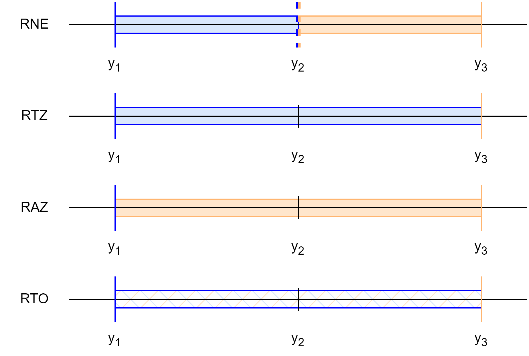
For each rounding mode, we color the interval $[y_1, y_3)$ with each segment (or tick) colored according to the rounding result: blue for $y_1$ and orange for $y_3$. Dual-coloring indicates a conditional rounding that depends on the value of $y_1$ (and $y_3$). RTO is dual-colored throughout; the midpoint $y_2$ is also dual-colored for RNE.

Notice that, for these rounding modes, we can distinguish four cases:

$x = y_1$: $x$ is representable, so all rounding modes produce $y_1$;
$y_1 < x < y_2$: $x$ is closer to $y_1$, so RNE and RTZ produce $y_1$, RAZ produces $y_2$; and RTO chooses based on parity of $y_1$;
$x = y_2$: $x$ is halfway, so RNE must tie-break based on parity, RTZ produces $y_1$, RAZ produces $y_2$; and RTO chooses based on parity of $y_1$.
$y_2 < x < y_3$: $x$ is closer to $y_3$, so RNE and RAZ produce $y_2$, RTZ produces $y_1$; and RTO chooses based on parity of $y_1$.

Analyzing these regions at precision $p + 1$, the significand of $y_1$ and $y_3$ are even, since increasing precision adds a trailing zero to their significands. For example, if $y_1 = 5/32$ with $p = 3$, then:

\[y_1 = 101 \cdot 2^{-5} = 1010 \cdot 2^{-6}.\]

By contrast, the significand of $y_2$ is odd. For the same example, the midpoint $y_2 = 11/64$ of $y_1$ and $y_3$ has the form

\[y_2 = 101.1 \cdot 2^{-5} = 1011 \cdot 2^{-6}.\]

The regions $(y_1, y_2)$ and $(y_2, y_3)$ are the intervals between adjacent representable numbers at precision $p + 1$. Recalling discussion from earlier, these regions are exactly the intervals represented by the sticky bit at precision $p + 2$. Therefore, rounding to odd at precision $p + 2$ results in four cases:

$x$ is exactly the endpoint $y_1$, so the last two digits of the rounded significand are $RS = 01$;
$x$ lies in $(y_1, y_2)$, so the last two digits of the rounded significand are $RS = 01$;
$x$ is exactly the midpoint $y_2$, so the last two digits of the rounded significand are $RS = 10$;
$x$ lies in $(y_2, y_3)$, so the last two digits of the rounded significand and $RS = 11$.

Notice that these cases correspond exactly to the four cases we identified earlier for standard rounding modes at precision $p$. After applying round to odd at precision $p + 2$, representable values (at precision $p$) are still representable; midpoints (at precision $p$) are still midpoints; and all other values, either on $(y_1, y_2)$ or $(y_2, y_3)$, are rounded to the midpoint of those intervals, preserving their nearness to one endpoint. Therefore, re-rounding under any standard rounding mode at precision $p$ yields the same result as rounding directly at precision $p$.

rounding $$x$$ between $$y_1$$ and $$y_3$$

Visually, we can indicate the round to odd step by overlaying gray arrows, representing round to odd at precision $p + 2$, over the previous figure. Layering the two rounding steps, we see that round to odd at precision $p + 2$ rounds values in $(y_1, y_2)$ or $(y_2, y_3)$ to the midpoints at precision $p + 1$; representable values and midpoints remain unchanged. Safe re-rounding corresponds to the coloring of the initial value $x$ being preserved after rounding to odd.

Therefore, round to odd at precision $p + 2$ preserves sufficient information so that we can safely re-round under any standard rounding mode at precision $p$. For precision $p + k$ where $k > 2$, the same reasoning applies: values that are neither representable nor midpoints may be rounded differently at precision $p + k$, but their nearness to one endpoint is preserved.

Applications

Boldo and Melquiond [2, 4] provide potential applications for round-to-odd. They include emulation of FMA, correctly-rounded addition of 3 terms, correctly-rounded sum of $n$ terms (under certain conditions), compiling the same constant under multiple precisions and rounding modes, and more.

More recent work relies on a corollary of Theorem 1. Combining the definition of a correctly-rounded function with Theorem 1, we get the following result:

\[\begin{align*} f^{*} &= \mathrm{rnd}^{p}_{rm} \circ f\\ &= (\mathrm{rnd}^{p}_{rm} \circ \mathrm{rnd}^{p+k}_{\text{RTO}}) \circ f\\ &= \mathrm{rnd}^{p}_{rm} \circ (\mathrm{rnd}^{p+k}_{\text{RTO}} \circ f)\\ &= \mathrm{rnd}^{p}_{rm} \circ f_{\text{RTO}}^{*}. \end{align*}\]

Stated otherwise, a correctly-rounded implementation of $f$ is the composition of (i) a round-to-odd implementation of $f$; followed by (ii) re-rounding under the desired rounding mode.

Corollary 2. Let $f$ be a real-valued function, and $f^{*}$ be a correctly-rounded implementation of $f$ at precision $p$ under rounding mode $rm$. If $f_{\text{RTO}}^{*}$ is a correctly-rounded implementation of $f$ at precision $p + k$ under round to odd ($k \geq 2$), then

\[f^{*} = \mathrm{rnd}^{p}_{rm} \circ f_{\text{RTO}}^{*}.\]

One successful application of this corollary is found in the RLibm project [5] which automatically generates efficient, correctly-rounded elementary functions by generating a polynomial approximation with additional bits of precision using round-to-odd arithmetic that will be correctly rounded when re-rounded under the desired rounding mode. The general principle of Corollary 2 suggests a modular approach to designing correctly-rounded functions for multiple precisions and rounding modes: first, design a round-to-odd implementation at higher precision; then, apply a re-rounding step to obtain the desired result.

Conclusion

This blog post covered the round to odd including its definitions, properties, and applications. Along the way, we learned about floating-point numbers, correctly-rounded functions, and how rounding works. The key property of round to odd, safe re-rounding, avoid double rounding and suggests a method for designing correctly-rounded functions by separating the concerns of approximating the infinitely precise result and rounding to the target number format. While round to odd is not widely supported in hardware or programming languages today, its unique properties make it a valuable techinique that should be better studied and more widely adopted.

References

IEEE. 2019. IEEE Standard for Floating-Point Arithmetic. IEEE Std 754-2019 (Revision of IEEE 754-2008), 1–84. DOI: https://doi.org/10.1109/IEEESTD.2019.8766229.
Sylvie Boldo, Guillaume Melquiond. When double rounding is odd. 17th IMACS World Congress, Jul 2005, Paris, France. pp.11. ffinria-00070603v2f.
Nicolas Brisebarre, Guillaume Hanrot, Jean-Michel Muller, and Paul Zimmermann. 2025. Correctly Rounded Evaluation of a Function: Why, How, and at What Cost?. ACM Comput. Surv. 58, 1, Article 27 (September 2025), 34 pages. https://doi.org/10.1145/3747840.
Sylvie Boldo and Guillaume Melquiond. 2008. Emulation of a FMA and Correctly Rounded Sums: Proved Algorithms Using Rounding to Odd. IEEE Transactions on Computers 57, 4 (2008), 462–471. https://doi.org/10.1109/TC.2007.70819.
Jay P. Lim and Santosh Nagarakatte. 2022. One Polynomial Approximation to Produce Correctly Rounded Results of an Elementary Function for Multiple Representations and Rounding Modes. Proc. ACM Program. Lang. 6, POPL, Article 3 (January 2022), 28 pages. https://doi.org/10.1145/3498664.

This work is licensed under a Creative Commons Attribution-ShareAlike 4.0 International License.

2025 2
2024 1
2021 4
2020 1

2025

Round to Odd

When writing numerical programs, rounding is a subtle but important aspect that can significantly affect the accuracy and stability of computations. In...

Composable, Correctly-Rounded Number Libraries

This blog post was split into two parts. This blog post covers rounding in detail and discusses some theory; this blog post focuses on design principles ...

2024

Rearchitecting Herbie’s improvement loop

Herbie’s improvement loop has five basic phases:

2020

First Entry

Note: This is my first entry for my blog, a compendium of my thoughts, articles, references, etc. Is blog even the correct word? I’m still trying to figure o...

Round to Odd

Floating-Point Numbers

Correctly-Rounded Functions

Rounding Modes

Round-to-Odd

Properties of Round-to-Odd

Applications

Conclusion

References

2025

Round to Odd

Composable, Correctly-Rounded Number Libraries

2024

Rearchitecting Herbie’s improvement loop

2021

A One-Year Retrospective on Minim

Garbage Collection in Minim

Developing Minim

Publishing the “generic-flonum” package

2020

First Entry